

Author: @atilayberber
Two things changed quietly in Fabric Data Warehouse during 2026. The first is how you pay: consumption is no longer tied to the CPU time a query burns, but to how long the compute allocated to your workspace (vNodes) stays up. The second is how that compute gets divided. On November 9, 2026 Microsoft announced that SQL pool configuration is being unified into a single model, and that new workspaces will start with a different default from January 2027.
Read together, they change what SQL pools are for. They used to be the “stop ETL from slowing my reports” setting. Now they are the main lever you have over warehouse consumption. This guide covers the architecture, the January 2027 timeline, setup through the portal and the API, ready-to-run T-SQL for monitoring, and the traps worth knowing about, with sources for every claim.
In short
- Warehouse and SQL analytics endpoint consumption is measured in vNodes (4 vCores each) with a one-minute baseline allocation window. Capacity Metrics now shows billing intervals, not individual queries.
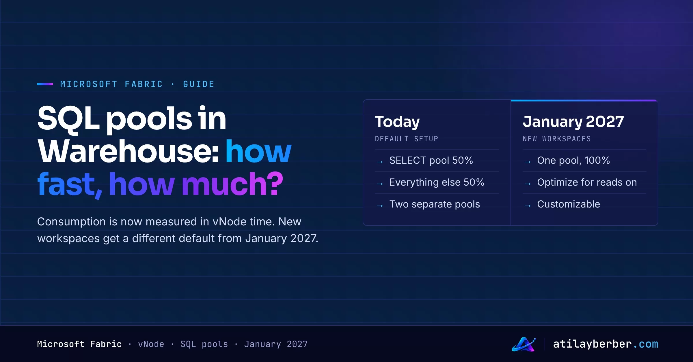
- By default, compute is split 50/50 between SELECT and non-SELECT workloads. Custom SQL pools let you design your own split, with up to 8 pools.
- From January 2027, new workspaces get a single read-optimized pool with access to 100% of compute. Active configurations on existing workspaces stay as they are.
- By mid-December 2026, any automation that relies on the
customSQLPoolsEnabledflag needs a review. - A pool percentage is not a budget cap. It is a guardrail on the maximum resources a workload can reach.
- Status: Microsoft’s “What’s new” page still lists custom SQL pools under preview; the statement type classifier went GA in September 2026; the REST API is beta.
Why this matters now
The billing logic moved from CPU time to allocated compute
The current consumption article on Microsoft Learn describes the model like this: Fabric allocates compute during read and write activity against a warehouse and read activity against a lakehouse’s SQL analytics endpoint. The unit is the vNode, a collection of four vCores. Resources are allocated using a one-minute baseline allocation window, then measured and reported per second based on the number of allocated vNodes. The article’s shorthand: Consumption = Active vNodes × Active Time.
The Fabric operations page states that one Data Warehouse core equals 0.538 CU. Put the two together and you can do some rough arithmetic (the math is mine, not a Microsoft price sheet):
- 1 vNode = 4 × 0.538 = 2.152 CU
- A 10-second query that wakes a single vNode shows up as roughly 60 × 2.152 = 129 CU-seconds because of the one-minute baseline.
- Twenty queries that fit in the same minute share that window, as long as they don’t need more vNodes.
Nikola Ilic (Data Mozart) reported, based on the notice Microsoft sent to customers, that this model took effect in August 2026 and replaced per-query CPU-time metering. His post is where the “one-minute trap” discussion started, and I won’t repeat it here. The question for this guide is different: under this model, which knobs do we actually have?
One practical consequence is on the monitoring side. Learn notes that the Operation Id in the Capacity Metrics app no longer maps to the distributed statement ID of warehouse queries. The app shows completed billing intervals; to find out what ran inside one, you query queryinsights.exec_requests_history with the interval’s start and end times. Queries on system catalog views and DMVs are billable too.
January 2027: a new default for new workspaces
According to Microsoft’s November 9 announcement, the distinction between built-in and custom pools is going away. All pools will be represented through one configuration model in the UI and the APIs, and new workspaces will start with one pool at 100% instead of today’s 50/50. Details below, after the architecture.
Architecture: how Fabric Warehouse shares compute
The default: autonomous workload management
Warehouse and the SQL analytics endpoint run on the same distributed SQL engine. Out of the box, the workspace’s compute is split evenly into two isolated pools: one for SELECT queries and one for ingestion and data modification (DML and DDL). Each scales independently with demand but never exceeds 50% of the total. The point is to keep a nightly load from starving report queries.
The ceiling comes from the capacity SKU. Warehouse can burst above baseline capacity; per the Learn table the burstable scale factor goes up to 12x for F8 through F2048, 32x on F2 and 16x on F4. In the autonomous setup that is managed as up to 12x per pool and 24x in total. Bursted consumption is then smoothed over time. I covered how smoothing and throttling work in Capacity Management in Fabric.
The scope is the workspace: every warehouse and SQL analytics endpoint in it shares the same pools.
Custom SQL pools: you draw the boundaries
With custom SQL pools, a workspace admin controls four things: how many pools exist, which requests go where, how much each pool can take at most, and whether a pool is optimized for reads.
| Aspect | Autonomous (default) | Custom SQL pools |
|---|---|---|
| Configuration | None, out of the box | Portal or REST API |
| Permission | Not applicable | Workspace Admin role |
| Number of pools | 2 (SELECT / other) | Up to 8 |
| Classification | Statement type | Statement type, application name, or application name regex |
| Resource share | 50% per pool | A percentage per pool; sum of 100% or less |
| Burst | Managed by Fabric (12x per pool, 24x total) | Shared by percentage; total is still 24x |
The attribute that routes a request to a pool is called a classifier. There are three types:
- Statement type: Creates exactly two pools (
SELECTandNONSELECT), each starting at 50%, with adjustable percentages. This is the part that went GA in September 2026. - Application name: Exact match on the application (program) name in the connection string. A pool can hold several names, a name is limited to 128 characters, and a name can’t appear in two pools.
- Application name regex: A regular expression matched against the application name. Only the first value in the list is evaluated. If a request matches the expressions of two pools, the pool is picked at random; there is no priority rule.
Two rules shape every design. A workspace can use only one classifier type, and exactly one pool must be the default, which catches everything that matches no rule.
“Optimize for reads” and cache cooldown
Every pool has an Optimize for reads option. Learn gives it one sentence: check it if you want the pool optimized for SELECT type queries. The unification announcement adds more. For ingestion-heavy workloads with limited cache reuse, turning it off avoids “unnecessary cache-related consumption”. And the default five-minute cache cooldown, the time compute stays allocated after activity, will be shortenable once it becomes configurable.
My reading (this is interpretation, not documentation): a read-optimized pool buys faster reports through a warm cache, and part of the price is idle minutes that still count as consumption. In a workspace that wakes up for sparse, short queries, that trade can go against you. The docs don’t quantify the effect, so you need to measure it in your own Capacity Metrics data.
What changes in January 2027?
| Scenario | What to expect |
|---|---|
| Existing workspace | Active pool configuration and workload behavior stay the same. Previously submitted but inactive configurations no longer appear in the UI or in GET responses. |
| New workspace (from January 2027) | One pool, Optimize for reads on, access to 100% of compute. You can customize it. |
| API integrations | The customSQLPoolsEnabled flag is removed. GET returns only the effective configuration; PATCH drops the flag while the pool payload stays the same. |
The timeline has two steps:
- By mid-December 2026: stop relying on
customSQLPoolsEnabledto retrieve inactive configurations. - Before the January 2027 rollout: remove logic that branches on built-in versus custom mode, and prepare for the flag disappearing from PATCH requests. Updated documentation is promised alongside the rollout.
The cost side is spelled out in the announcement and applies to new workspaces only. Both SELECT queries and ingestion will be able to reach 100% of available compute instead of today’s 50% each. That can mean faster completion and higher compute consumption. Microsoft suggests three brakes: give pools smaller percentages, turn off Optimize for reads for ingestion-heavy work, and shorten the cooldown once that setting ships.
How I read it: nothing breaks in your current environment. But every workspace you create after January will be born with a different consumption profile than the ones you have today. If you create workspaces from a template or through automation, pool configuration belongs in that template.
Step by step
1. Start with an inventory: who connects, and under what name?
Look at the traffic before you design anything. queryinsights.exec_requests_history records program_name (the application name) and sql_pool_name (the pool that ran the request) for every completed request. Query Insights keeps 30 days of history, and a query can take up to 15 minutes to appear.
SELECT
    program_name,
    sql_pool_name,
    statement_type,
    COUNT(*)                             AS request_count,
    SUM(allocated_cpu_time_ms) / 1000.0  AS vcore_seconds,
    SUM(data_scanned_remote_storage_mb)  AS onelake_mb,
    SUM(data_scanned_memory_mb + data_scanned_disk_mb) AS cache_mb
FROM queryinsights.exec_requests_history
WHERE start_time >= DATEADD(DAY, -14, GETUTCDATE())
GROUP BY program_name, sql_pool_name, statement_type
ORDER BY vcore_seconds DESC;
The output answers three questions: which application names really exist, which ones use the most resources, and which ones benefit from the cache (high onelake_mb with low cache_mb means the cache isn’t doing much). sql_pool_name is empty for lightweight queries that don’t need distributed execution. That is expected.
With the one-minute window in mind, a second view helps: in how many distinct minutes per hour did a query start?
SELECT
    CAST(start_time AS date)        AS activity_date,
    DATEPART(HOUR, start_time)      AS activity_hour,
    COUNT(DISTINCT DATEDIFF(MINUTE, '2026-01-01', start_time)) AS minutes_with_query_start,
    COUNT(*)                        AS request_count
FROM queryinsights.exec_requests_history
WHERE start_time >= DATEADD(DAY, -7, GETUTCDATE())
GROUP BY CAST(start_time AS date), DATEPART(HOUR, start_time)
ORDER BY activity_date, activity_hour;
Hours where a handful of requests “wake” many separate minutes point to sparse, scattered traffic. This query only counts start minutes. It doesn’t calculate a bill; it tells you where to look.
2. Design the pools
Decide in this order:
- Classifier type. If all you want is a different read/write ratio, statement type is enough. To separate applications you need application name. For traffic whose name contains variable parts such as GUIDs (Fabric pipelines, for example), you need regex.
- Default pool. Everything you don’t recognize lands here. Making your broadest, most critical traffic the default keeps a forgotten application from being squeezed into a narrow pool.
- Percentages. The sum can’t exceed 100%, but it doesn’t have to reach 100% either. Keeping the total deliberately low is exactly what Learn recommends in its capacity throttling scenario.
- Optimize for reads. On for repetitive report queries and off for load pools is a reasonable starting point.
Learn provides ready-made values for Fabric’s own traffic:
- Fabric pipelines:
^Data Integration-to[0-9a-fA-F]{8}-[0-9a-fA-F]{4}-[1-5][0-9a-fA-F]{3}-[89abAB][0-9a-fA-F]{3}-[0-9a-fA-F]{12}$ - Power BI:
^(PowerBIPremium-DirectQuery|Mashup Engine(?: \(PowerBIPremium-Import\))?) - The SQL query editor in the Fabric portal:
DMS_user
3. Set it up in the portal
- In the workspace, open Workspace settings, expand Data Warehouse and go to the SQL Pools page. On the default setup the page says Using built-in pools.
- Select Set up custom pools.
- Pick the Classifier type: Application name (exact name), Application name (regex) or Statement type.
- The first pool is generated automatically and is the default pool, which is why its application name field is disabled. Enter the Pool name and Compute %, and check Optimize for reads if needed.
- Add the other pools with + New SQL Pool, giving each a unique name, classifier value and percentage.
- Save. To go back, use Revert to built-in setup on the same page.
4. Set it up through the API (the repeatable way)
The API is the better fit when the same configuration has to travel across environments. The example below is adapted from the notebook sample on Learn and runs in a Fabric notebook. The endpoint is beta today, hence the ?beta=true parameter.
import json
import requests
from notebookutils import mssparkutils

workspace_id = mssparkutils.runtime.context.get('currentWorkspaceId')
url = (
    f'https://api.fabric.microsoft.com/v1/workspaces/{workspace_id}'
    '/warehouses/sqlPoolsConfiguration?beta=true'
)
headers = {'Authorization': f'Bearer {mssparkutils.credentials.getToken("pbi")}'}

# 1) Read and keep the current state
current = requests.get(url, headers=headers)
print(json.dumps(current.json(), indent=4))

# 2) New configuration
body = {
    "customSQLPoolsEnabled": True,
    "customSQLPools": [
        {
            "name": "reporting",
            "isDefault": True,
            "maxResourcePercentage": 50,
            "optimizeForReads": True
        },
        {
            "name": "etl",
            "isDefault": False,
            "maxResourcePercentage": 35,
            "optimizeForReads": False,
            "classifier": {
                "type": "Application Name",
                "value": ["etl-nightly", "etl-hourly"]
            }
        },
        {
            "name": "adhoc",
            "isDefault": False,
            "maxResourcePercentage": 15,
            "optimizeForReads": False,
            "classifier": {
                "type": "Application Name",
                "value": ["DMS_user"]
            }
        }
    ]
}

response = requests.patch(url, json=body, headers=headers)
print(response.status_code, response.text)
Things to know:
- Unless
customSQLPoolsEnabledistrue, the payload is ignored and autonomous management stays in place. The flag disappears with unification; keeping it on a single line makes it easy to delete in January. - PATCH replaces the whole list. In the words of the semantic-link-labs documentation, any existing pool not included in the request is deleted. Save the GET output first.
- To revert:
{"customSQLPoolsEnabled": false, "customSQLPools": []}. - If you’d rather not call REST directly, semantic-link-labs wraps the same API in
sempy_labs.warehousewithget_sql_pools_configuration,enable_sql_pools_configurationanddisable_sql_pools_configuration, and supports service principals.
5. Verify
You can confirm the application name arrives by checking live sessions:
SELECT session_id, program_name
FROM sys.dm_exec_sessions
WHERE program_name = 'etl-nightly';
After 10 to 15 minutes, Query Insights shows which pool the request landed in:
SELECT distributed_statement_id, submit_time, program_name,
       sql_pool_name, start_time, end_time
FROM queryinsights.exec_requests_history
WHERE program_name = 'etl-nightly'
ORDER BY submit_time DESC;
End-to-end example: three workloads, one workspace
The scenario is made up, and the percentages are a starting point rather than a recommendation.
A workspace carries three kinds of traffic: Power BI reports (DirectQuery and import refreshes), a nightly load service written in Python, and analysts working in the portal’s query editor. The complaint is a familiar one: a heavy analyst query slows down the morning reports, and the nightly load pushes the capacity.
Design decisions:
- The load service is our own code, so we control the application name in its connection string. The query editor’s name is documented (
DMS_user). Both can be caught by exact name, so we pick the Application name type. - Power BI’s names vary, so we don’t classify it at all. We make
reportingthe default pool instead, and everything unclassified falls into it. reportinggets 50% and is read-optimized;etlgets 35% and isn’t;adhocgets 15%.
In the load service, adding the application name to the connection string is all it takes. The keyword is APP for the ODBC driver and Application Name for .NET SqlClient:
conn_str = (
    "Driver={ODBC Driver 18 for SQL Server};"
    "Server=<your-sql-connection-string>;"
    "Database=<warehouse-name>;"
    "APP=etl-nightly;"
    "Encrypt=yes;"
    # add the authentication parameters your environment uses
)
A week later, the first place to look is pressure. queryinsights.sql_pool_insights writes a row whenever pool configuration, capacity or pressure state changes. A pressure change is logged only if it lasts a minute or longer.
SELECT [timestamp], sql_pool_name, max_resource_percentage,
       is_optimized_for_reads, current_workspace_capacity,
       is_pool_under_pressure
FROM queryinsights.sql_pool_insights
WHERE is_pool_under_pressure = 1
  AND [timestamp] > DATEADD(WEEK, -1, GETDATE())
ORDER BY [timestamp] DESC, sql_pool_name;
To see what was running during pressure, this is the pattern from Microsoft’s SQL Pool Insights announcement:
WITH Pool_Pressure_Events AS (
    SELECT DISTINCT [timestamp]
    FROM queryinsights.sql_pool_insights
    WHERE is_pool_under_pressure = 1
)
SELECT erh.sql_pool_name, erh.program_name, erh.start_time,
       erh.total_elapsed_time_ms, erh.allocated_cpu_time_ms, erh.command
FROM queryinsights.exec_requests_history AS erh
JOIN Pool_Pressure_Events AS ppe
  ON ppe.[timestamp] BETWEEN erh.start_time AND erh.end_time
ORDER BY erh.allocated_cpu_time_ms DESC;
Then decide. If adhoc is constantly under pressure and that’s acceptable (an analyst query waits a little), leave it alone; that is the pool doing its job. If reporting is under pressure, move share to it from etl or adhoc. Changing a percentage doesn’t fail running queries.
Finding the expensive interval: from Capacity Metrics into the warehouse
The Monitor in warehouse action, generally available since early November 2026, connects the capacity view straight to Warehouse Monitor. In Capacity Metrics you pick a timepoint on the Compute page, select Explore to open TimePoint Detail, choose a warehouse query operation under background operations, and select Monitor in warehouse. The warehouse opens with the time window already applied. You need access to the Capacity Metrics app and the Admin role in the warehouse’s workspace.
Microsoft’s advice is to sort by CPU time and read Data scanned, Result cache hit, Label and Is distributed together. The same post carries an important caveat: CPU time is not the CUs billed for an individual query. So this screen doesn’t answer “which query was expensive?” It answers “who was keeping the compute busy during that interval?” For persistent, workspace-level monitoring, see the Workspace Monitoring guide.
Pitfalls and troubleshooting
- Deleting a pool cancels running queries. A query running on a removed pool fails with “Query canceled by user”. Resizing does not. Make structural changes outside the load window.
- Scaling down can leave a pool with nothing. Pools rescale automatically when the SKU changes, but if downscaling forces a pool to zero nodes, queries fail with “The assigned SQL pool for this query has no resources and must be reconfigured.” Watch for this with small percentages on small SKUs.
- Regex overlap is silent. If two pools’ expressions match the same request, the choice is random and nothing errors. Anchor expressions with
^and$, and check with the verification query. - One classifier type. You can’t define one pool by statement type and another by application name in the same workspace. If you need both, split the workloads across workspaces.
- An empty
sql_pool_nameis fine. Queries that don’t need distributed execution aren’t assigned to a pool. - Expect gaps in the log.
sql_pool_insightsonly logs while the warehouse is active. - The scope is the workspace. Pools cover every warehouse and SQL analytics endpoint in it. If a Direct Lake model falls back to DirectQuery, those queries draw from the same compute; I covered fallback in the Direct Lake post.
- The API is beta. The contract can change, and January’s unification is a concrete example.
Governance and cost notes
A percentage is not a budget. Microsoft’s own blog post on the topic says so directly: pools are not spending limits or budget caps, they are guardrails on the maximum resources a workload can access. Putting a latency-insensitive load into a narrow pool means it runs longer and consumes resources at a smoother rate. It doesn’t guarantee a bill; it flattens peaks.
Workspace sprawl is now a cost topic. Because the one-minute baseline applies per workspace, the same small queries spread over ten workspaces are not equivalent to running them in one; Nikola Ilic shows this with worked examples. At the same time, Learn recommends using the workspace as an isolation boundary. So the workspaces you split for security and ownership may carry a consumption cost. Make that trade knowingly.
Inventory across many workspaces. Pools are configured per workspace, so “which ones are still on the default?” can’t be answered by hand across hundreds of them. A notebook published on GitHub by Microsoft’s Mark Pryce-Maher loops over every workspace and writes the configuration to Delta tables; by default it only reads (DRY_RUN). It is an MIT-licensed sample, not an official product, so try it on a test workspace first.
Who can change it? Only the workspace Admin role. One more reason to review how many admins your production workspaces have.
I discussed the wider trade-offs of the capacity model in Fabric Throttles, Databricks Bills. SQL pools are a new control on the Fabric side of that argument.
Checklist
Before January 2027:
- Do any scripts, pipelines or tools call the SQL pools API? Find every place
customSQLPoolsEnabledappears. - If you need old inactive configurations, retrieve and store them with GET before mid-December.
- Add a pool configuration step to your workspace creation process (template, script, CI/CD).
- Make a deliberate Optimize for reads decision for ingestion-heavy workspaces.
For each workspace:
- Run the inventory query: application names, resource use, cache ratio.
- Choose the classifier type and the default pool.
- Assign percentages and document the reasoning behind the total.
- Save the GET output, then apply.
- After 15 minutes, verify with
sql_pool_name. - After a week, review
sql_pool_insightsand Capacity Metrics.
Wrapping up
On their own, SQL pools look like a performance setting. Next to vNode-based consumption and the January 2027 default, they become the place where you balance how fast against how much. Your existing workspaces stay put. What changes is every workspace you create from here on, and your automation.
Which setup are you on: the default 50/50, or your own pools? Did you see a difference in consumption after turning off Optimize for reads? Tell me on LinkedIn; I’d like to see real measurements.
Sources
- Unifying SQL Pools: Upcoming changes to UI and APIs – Microsoft Fabric Updates Blog (November 9, 2026)
- Custom SQL pools – Microsoft Learn
- Configure custom SQL pools in the Fabric portal – Microsoft Learn
- Configure custom SQL pools by using the Fabric REST API – Microsoft Learn
- Workload management – Microsoft Learn
- Warehouse consumption and utilization – Microsoft Learn
- Burstable capacity in Fabric Data Warehouse – Microsoft Learn
- Fabric operations (CU rates) – Microsoft Learn
- queryinsights.exec_requests_history – Microsoft Learn
- queryinsights.sql_pool_insights – Microsoft Learn
- Query insights – Microsoft Learn
- What’s new in Microsoft Fabric – Microsoft Learn
- Find expensive queries from Capacity Metrics (GA) – Microsoft Fabric Updates Blog
- Using Custom SQL Pools to balance performance and cost in Fabric Data Warehouse – Microsoft Fabric Updates Blog
- Introducing SQL Pool Insights in Microsoft Fabric Data Warehouse – Microsoft Fabric Updates Blog
- One-minute trap! How new Fabric Warehouse CU metering affect your workloads – Nikola Ilic, Data Mozart
- sempy_labs.warehouse – semantic-link-labs documentation
- fabric-sql-pools-config – Mark Pryce-Maher, GitHub